Build Models on Massively Big Data using Continuous/Online Learning

The world seems to be in some mad race in accumulating more data by the day. The rate of data growth is being measured in zetta bytes. With this mammothic data accumulation, comes mammothic task of managing them and use them for model building. A lot of times, it gets difficult to preview such data, let alone do any operations on them. Below, I’ve listed a few steps on how not to get overwhelmed by this scale. I would be using the data from Kaggle — Click Through Rate Prediction Competition for most of the examples and illustrations.

Preview the data:

Most of us get comfortable only when we preview the data, before we start analyzing and building models . Like Andrej Karpathy says:

The first step to training a neural net is to not touch any neural net code at all and instead begin by thoroughly inspecting your data. This step is critical. I like to spend copious amount of time (measured in units of hours) scanning through thousands of examples, understanding their distribution and looking for patterns. Luckily, your brain is pretty good at this.

But when you are presented with a few gigabytes of data in a single file, it gets harder to open/preview the data using traditional tools like notepad++ or vim, which consumes the entire system RAM to load the files. One alternative is to use tools like less in UNIX, which helps us just get the preview of the data instead of loading the entire data. In Windows, there are options like EditPad Lite and Large Text File Viewer, although, I still prefer the using the more command from the powershell or even better, using all the benefits of Unix from WSL. Below if the data preview by running a less command on the train.csv from the CTR prediction dataset:

Once we preview the data visually, we at least know the basic traits of the file like the number of columns, column names (if present as a part of the header), delimiter, basic types of the fields (numeric, floating, string, etc.), presence of missing values (if you can capture it in the first few records). You could also compute the total records by wc -l command (word count)

Read Data

The next logical step would be to read this data into your system. Again, given the massive data size, it would be close to impossible to read the dataset into the system RAM.

Read Data line by line:

One option would be to read it line by line as per the example given below. Note: I have not added any preprocessing, but one may choose to perform any processing after the read step (at the comment). Also note that, the above code will read every variable as string. One may want to do necessary type conversions in the processing step.

This works well without running into any RAM constraints, and it takes about 70 seconds to read 5 .8 GB of data. This method will work in any data size, in any given system RAM.

Read Mini-Batch Data with Pandas:

While the above method works perfectly well on any small machine, we can see that it is pretty inefficient, as it processes line after line. This has two problems:

• We are not utilizing the complete RAM of the system and we can definitely do better on time
• Some of the data processing may require us to see more than 1 line of data (for example finding out the distribution of a variable)

This can be addressed by mini-batch read. One easiest way to read the data in minibatch would be to use chunksize in pandas.read_csv module as shown below.

You could also choose the columns that you wish to read, by specifying usecols option in read_csv, thus reducing the memory consumption even further.

Dask

Another alternative is to use dask, which utilizes clever distributed computing and lazy loading. This means that it uses multiple cores to read the data in parallel, and at times when when you run short of memory, it only loads the structure of the data and returns the actual data only when required. In the below example, you can see that it hardly takes a few micro-seconds to perform read_csv.

The below code summaries all the three approaches:

import time
	import pandas as pd
	import dask.dataframe as dd
	class read_data:
	def __init__(self, file_path:str):
	self.file_path = file_path
	def process_data_linebyline(self):
	start_time = time.time()
	with open(self.file_path,’r’) as f:
	for n,line in enumerate(f):
	if n > 0: #ignore the header
	data = line.rstrip().split(‘,’)
	#further process data
	print(” — %s seconds –” % (time.time() – start_time))
	def process_data_dataframechunks(self,chunksize : int):
	start_time = time.time()
	df = pd.read_csv(self.file_path,chunksize=chunksize)
	for chunk in df:
	pass
	#further process chunks
	print(” — %s seconds –” % (time.time() – start_time))
	def process_data_dask(self):
	dtype_dict = {
	‘id’:’uint64′,
	‘click’:’int64′,
	‘hour’:’int64′,
	‘C1′:’int64’,
	‘banner_pos’:’int64′,
	‘site_id’:’object’,
	‘site_domain’:’object’,
	‘site_category’:’object’,
	‘app_id’:’object’,
	‘app_domain’:’object’,
	‘app_category’:’object’,
	‘device_id’:’object’,
	‘device_ip’:’object’,
	‘device_model’:’object’,
	‘device_type’:’int64′,
	‘device_conn_type’:’int64′,
	‘C14′:’int64’,
	‘C15′:’int64’,
	‘C16′:’int64’,
	‘C17′:’int64’,
	‘C18′:’int64’,
	‘C19′:’int64’,
	‘C20′:’int64’,
	‘C21′:’int64’
	}
	start_time = time.time()
	df = dd.read_csv(self.file_path, dtype=dtype_dict)
	print(” — %s seconds –” % (time.time() – start_time))
	print(df.head())
	if __name__ == “__main__”:
	readObj = read_data(‘../data/train.csv’)
	#readObj.process_data_linebyline()
	#readObj.process_data_dataframechunks(chunksize=500000)
	readObj.process_data_dask()

Numpy memmap

Speaking about lazy loading, if you happen to have only numeric data, then we can alternatively make use of numpy memmap, which only maps the addresses of the data on the disk. It actually fetches the data only when it is referenced with the indices when required. (https://stackoverflow.com/questions/43393821/how-to-concat-many-numpy-arrays)

ftrainY = np.memmap('data/trainY.npy',dtype=np.int,shape=(15727857,),mode='w+')
ftestY = np.memmap('data/testY.npy',dtype=np.int,shape=(3931965,),mode='w+')fread = np.memmap('data/trainY.npy',mode='r',shape=(15727857,))def chunker(seq, size):
    return (seq[pos:pos + size] for pos in range(0, len(seq), size))for batch in chunker(fread,500000):
    print(batch.mean())

Database based alternatives

Other ways to read such massive data would be to create a mini database like sqlite in your own system and use tools like sqlalchemy to read them with filters, etc. I’ll probably reserve that discussion for another post.

Building Models

Once the data is loaded, the next task would be to perform some variable reduction or some modelling. A lot of the readily available machine learning packages mostly expect the entire data to be loaded into the RAM for performing their ‘fit’ functions. Below I’ll illustrate some of the ways to ensure that the ‘fit’ happens irrespective of the data size.

Smarter Initialisers leads to faster convergence

A lot of algorithms are sensitive to the weight initialisers. A purely random weight initialisation would take a longer duration to converge as it will have to re-adjust its weights a lot more to the optimal points. Also poor initialisation may lead to exploding/vanishing gradients. There are smarter hacks to intelligently initialise your weights before beginning to learn. For example, if we are trying to perform a regression whose mean value is say — 250, then initialise your bias to be equal to 250. Also scale your input variables before fitting, so as to reduce the range of gradients while learning. For classification problems, initialise the logit bias such that your model predicts probability equal to the 1:0 ratios at initialisation. While clustering, determine the distribution of points by various features (Eg: get the 5th, 10th, 25th, 50th, 75th, 90th and 95th percentiles of each features) and initialise the centroids around these ranges.

Another alternative could be to fit a model on a very small sample and use these weights (in case of supervised models) OR centroids (in case of unsupervised models) as initialisers for the large dataset modelling.

Partial/Incremental fit vs full fit

A lot of the algorithms allow stochastic learning. That means, instead of learning from the entire data, they can learn if they were provided row-by-row data. This could even be extended to a mini-batch data (a small set of rows, instead of single row). That means, in a typical supervised learning setup, we start with some randomly assigned — learnable weights, and keep adjusting those weights as and when we encounter more data and labels. Below, I shall discuss some of the methods that uses these partial fit/incremental fit —

Data Scaling:

The data can be across different units of measurements (like percentages, large float numbers, small ranged integers, binary, etc.). In order to bring all these variables to a comparable scale, we perform scaling. The most popular API for scaling is StandardScaler or MinMaxScaler. StandardScaler computes the Mean/Standard Deviation of the variables and subtracts the mean from each row of the variable and divides it with the Standard Deviation, thus ensuring that distribution of the variable has a mean of 0 and standard deviation of 1. i.e. —

where μ is the mean of the variable and σ is the standard deviation of the variable.

Similarly, the MinMax Scaling is performed by taking the ratio of the difference of each row of the variable with that of the min value of the variable to the difference max value of the variable with that of each row of the variable. i.e. —

However, both the StandardScaler and the MinMax Scaler in the above equations will require the entire distribution to be made available at once (in order to compute the mean, standard deviation, max and min). But we still are stuck with the big data problem of not being able to load the entire data into the memory. In order to circumvent this, we employ incremental aggregation computation methods, which will compute the mean, standard deviation, min and max incrementally. Though this may not result in accurate values, these approximations usually hold well for the large data.

Incremental Mean:

• We know that a simple mean of a variable is expressed as the sum of the variable values divided by the number of observations

• By re ordering some of the terms as given below, we can express the mean of the variable upto the n-th observation as a function of the the mean upto the n-1 th observation

Thus, you can see that the mean for the n-th observation can be derived from the n-1 th observation. In other words, the mean of a variable can be calculated incrementally. Similarly, we can also show that the standard deviation too, can be calculated incrementally. And so is the min and max of a variable (keep a pseudo min/ max variable and keep reassigning that variable as and when you encounter the new min and new max in the variable observations).

Using the above incremental aggregation concept, scikit learn has enabled a partial fit function for both the scaler, which keeps learning the scale function everytime you pass a chunk of data to it. So the learning can be done chunkwise. Once the entire data is fit, you can use the scaler object for further transformations. Below code shows how it can be done —

import pandas as pd
	from sklearn.preprocessing import StandardScaler, MinMaxScaler
	chunksize = 100000
	stdscaler = StandardScaler()
	#Consider only numeric drivers for our example
	numeric_drivers = [‘hour’,’banner_pos’,’C1′,’device_type’,’device_conn_type’,’C14′,’C15′,’C16′,’C17′,’C18′,’C19′,’C20′,’C21′]
	df = pd.read_csv(‘../data/train.csv’,chunksize=chunksize)
	for chunk in df:
	stdscaler.partial_fit(chunk[numeric_drivers])
	#continue preprocecssing

Dimension Reduction:

• Principal Component Analysis is typically used to reduce the large dimension to smaller components, where each of these components are expressed as a linear function of all the underlying features, while ensuring that each of these linear components are orthogonal to each other. I would not delve more into the working of PCA as such, but would point out that there exists an IncrementalPCA API in the sklearn library. This takes in the data batch-by-batch and incrementally fits the Components, which turns out to be pretty useful while training a large data. Below is an example usage of IncrementalPCA on the same large data example. Note that we also scale the data before we fit the PCA.

	import pandas as pd
	import numpy as np
	from sklearn.preprocessing import StandardScaler, MinMaxScaler
	from sklearn.decomposition import IncrementalPCA, PCA
	from matplotlib import pyplot as plt
	chunksize = 10000
	numeric_drivers = [‘hour’,’banner_pos’,’C1′,’device_type’,’device_conn_type’,’C14′,’C15′,’C16′,’C17′,’C18′,’C19′,’C20′,’C21′]
	df = pd.read_csv(‘../data/train.csv’,usecols=numeric_drivers,nrows=1000000)
	#Perform scaling
	stdscaler = StandardScaler()
	df = stdscaler.fit_transform(df)
	#fit the Incremental PCA
	pcainc = IncrementalPCA(n_components=len(numeric_drivers),batch_size=10000,copy=False,whiten=True)
	pcainc.fit(df)
	#find components that are explaining more than 85% of the variance
	print(np.where(pcainc.explained_variance_ratio_.cumsum()<=0.85)[0].shape)
	#plot the explained variance chart
	plt.plot(range(0,len(numeric_drivers)),pcainc.explained_variance_ratio_,’bx-‘)
	plt.xlabel(‘# Principal Components’)
	plt.ylabel(‘Explained Variance’)
	plt.title(‘Determine the # of PrinComps using explained variance’)
	plt.show()
	#plot the cumulative explained variance chart
	plt.plot(range(0,len(numeric_drivers)),pcainc.explained_variance_ratio_.cumsum(),’bx-‘)
	plt.xlabel(‘# Principal Components’)
	plt.ylabel(‘Total Explained Variance’)
	plt.title(‘Determine the # of PrinComps using explained variance’)
	plt.show()

• AutoEncoders: Any neural network based method will naturally allow stochastic OR minibatch learning. It requires us to use the fit method (earlier known as the fit_generator, now overloaded into fit), by passing in a data generator instead of the actual data. In the next section, I’ve shown a sample — generic data generator, that could be used for any data, and also built a sample autoencoder that can compress the dimensions, similar to a PCA. More discussions on how an AutoEncoder compares to a PCA is outside the scope of this post — so probably another post on this..
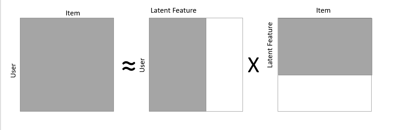
• Incremental Matrix Factorization: Matrix Factorization is a popular method that is used not only in dimension reduction, but also in recommender systems, generating user/item embeddings, etc. The latent dimension that is generated out of the matrix factorization an be used as the reduced set of dimensions that represents the matrix as shown in the figure below. The typical set up requires us to load the entire response matrix to the RAM and perform the matrix decomposition which gets very expensive as the data and the sparsity increases. Alternatively, one can use a stochastic learning framework to learn the responses using any common algorithm like Alternating Least Squares, etc. to Factorize the Matrix, thus, being able to decompose any large matrix, with smaller RAM size. One such application is explained well in Incremental SGD (ISGD) — J. Vinagre, et al., 2014. Below is a small snippet that can perform such incremental sgd in a simple response matrix setup

import numpy as np
	class incrementalSGD:
	def __init__(self, n_users, n_items, n_factors, alpha = 0.001, l2 = 0.01) -> None:
	self.n_users = n_users
	self.n_items = n_items
	self.n_factors = n_factors
	self.alpha = alpha
	self.l2 = l2
	self.user_latent = np.random.normal(0., 0.1, (self.n_user, self.n_factors))
	self.item_latent = np.random.normal(0., 0.1, (self.n_items, self.n_factors))
	def factorize(self, user_index, item_index, response):
	user_vector = self.user_latent[user_index]
	item_vector = self.item_latent[item_index]
	err = response – np.inner(user_vector, item_vector)
	self.user_latent[user_index] = user_vector + self.alpha * (err * item_vector – self.l2 * user_vector)
	self.item_latent[item_index] = item_vector + self.alpha * (err * user_vector – self.l2 * item_index)

view raw

Clustering:

A lot of partial fit based algorithms are made available that can incrementally learn the homogeneous groups of observations and add them to the clusters. Some of the examples include MiniBatchKMeans and Birch.

MiniBatchKMeans randomly samples mini batches of observations during each iterations during the training. At the initial iterations, the centroids are created local to the sampled space, thus leading to major updates in the centroids as and when we sample different spaces over subsequent iterations. After enough number of iterations, this would converge to the true universal centroids. In order to decrease the major updates to the centroid at each iterations, owing to the random samples, one hack could be to update the centroids by taking an incremental average (there we go again!!) of the current centroid position with respect to all the previous mini batches.

Birch on the other hand, creates trees called as Clustering Feature Tree, which can be treated as a lossy compression. The leaf nodes can then be treated as centroids. For more details, I recommend this blog by Cory Maklin which is quite intuitive to understand.

The codes for partial_fit for MiniBatchKMeans and Birch are well documented in the scikit-learn site.

Classification/Prediction:

Supervised learning can be performed either using Stochastic Gradient Descent’s partial fit or by using the incremental least squares (Code given below). The idea is similar, where we read mini batch observations and try adjusting the weights stochastically. Scikit-learn has a bunch of algorithms like SGDRegressor, SGDClassification, MultiNomialNB and BernoulliNB (Naive Bayes), PassiveAgressiveClassifier, Perceptron.

One can also tweak the LeastSquare algorithm to incrementally update the co-variance matrix, that can enable us to partially fit the data. Below is a code that I found on stackexchange, which does this —

import pandas as pd
	import numpy as np
	file_path = ‘../data/train.csv’
	chunksize = 1024
	X_vars = [‘hour’,’banner_pos’,’C1′,’device_type’,’device_conn_type’,’C14′,’C15′,’C16′,’C17′,’C18′,’C19′,’C20′,’C21′]
	y_var = ‘click’
	meanX = np.zeros((chunksize,len(X_vars)))
	meanY = np.zeros(chunksize)
	varX = 0
	covXY = 0
	meanXY = 0
	varY = 0
	alpha=0.001
	betas = np.zeros(len(X_vars))
	df = pd.read_csv(file_path,chunksize=chunksize)
	c = 0
	for chunk in df:
	X = chunk.loc[:,X_vars]
	y = chunk.loc[:,y_var]
	dx = X – meanX
	dy = y – meanY
	dxy = (X*y) – meanXY
	varX += ((1-alpha)*dx*dx – varX)*alpha
	varY += ((1-alpha)*dy*dy – varY)*alpha
	covXY += ((1-alpha)*dx*dy – covXY)*alpha
	meanX += dx * alpha
	meanY += dy * alpha
	meanXY += dxy * alpha
	betas = covXY/varX
	bias = meanY – np.dot(betas,meanX)

Tensorflow too, supports fitgenerator (now overloaded with fit function itself), where once can write a generator method to push the data in a streaming fashion for mini-batch stochastic learning. Tensorflow has a ready implemented image generator. Below is an implementation of a sample custom fitgenerator.

import numpy as np
	def generator(X_data, y_data, batch_size):
	samples_per_epoch = X_data.shape[0]
	number_of_batches = samples_per_epoch/batch_size
	counter=0
	while 1:
	indices = list(range(batch_size*counter,min(batch_size*(counter+1),samples_per_epoch)))
	np.random.shuffle(indices)
	X_batch = np.array(X_data[indices]).astype(‘float32’)
	y_batch = np.array(y_data[indices]).astype(‘int’)
	counter += 1
	yield X_batch,y_batch
	#restart counter to yeild data in the next epoch as well
	if counter >= number_of_batches:
	counter = 0
	batch_size = 512
	history = tfmodel.fit_generator(
	generator(trainX,trainY,batch_size),
	epochs=10,
	steps_per_epoch = trainX.shape[0]/batch_size,
	validation_data = generator([testX,testY,batch_size),
	validation_steps = testX.shape[0]/batch_size
	)

Conclusion

In summary, do not get bogged down by the size of the data. Bring on all the data in the world and with the right set of tools (both mathematical and computational) and the Attitude to solve them, we should be able to take on any monster to tackle.

Let me know your comments and thoughts.

Originally published on Medium